Data132.xls

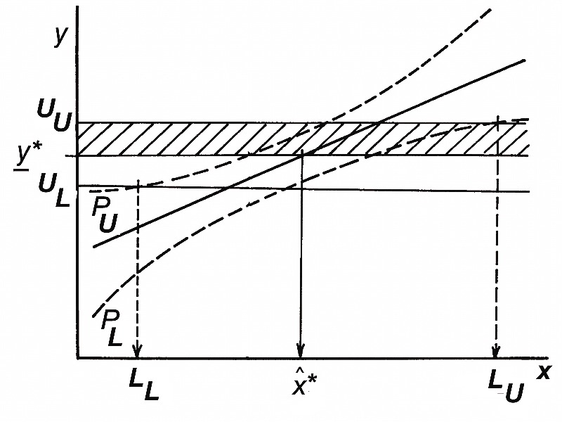
Fig. 1 Determination of the confidence interval of the concentration x for a calibration straight line: the absolute calibration and a procedure for determination x* for the mean value of analytical signal response y * being referred with the horizontal line and the confidence intervals of the signal of concentration, and f(x, b) is the predicted calibration straight line with its confidence intervals for a predicted observation. The horizontal x axis refers to the concentration and the vertical y axis to the signal response.

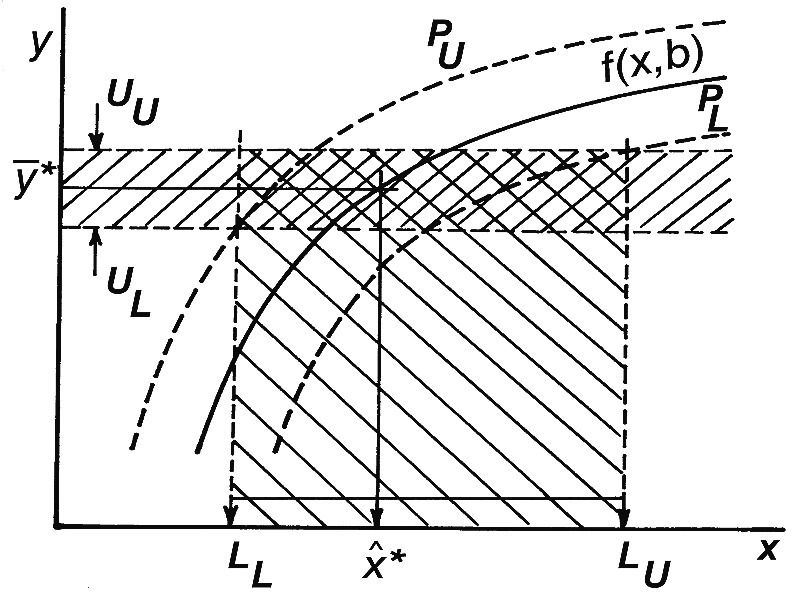
Fig. 2 Determination of the confidence interval of the concentration x for a nonlinear calibration curve: the absolute calibration and a procedure for determination x* for the mean value of analytical signal response y* being referred with the horizontal line and the confidence intervals of the signal indicated by the hatched area. LL and LU are the lower and upper limits of the confidence interval of concentration, and f(x, b) is the predicted calibration curve with its confidence intervals for a predicted signal response. The horizontal x axis refers to the concentration and the vertical y axis to the signal response.

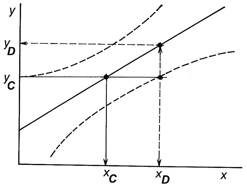
Fig. 3 Calibration design of the critical level in the response yC and the concentration xC units and the detection limit yD and corresponding concentration xD units. It includes the calibration straight line and Working-Hotteling confidence bands, cf. page 22 in ref. [50].

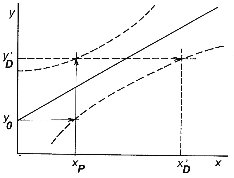
Fig. 4 The graphical procedure for determination of the detection limit yD and xD according to Ebel and Kamm [18].

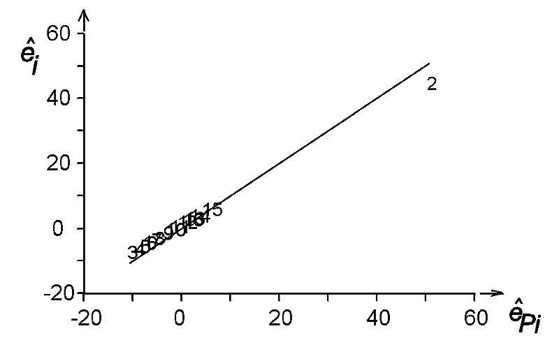
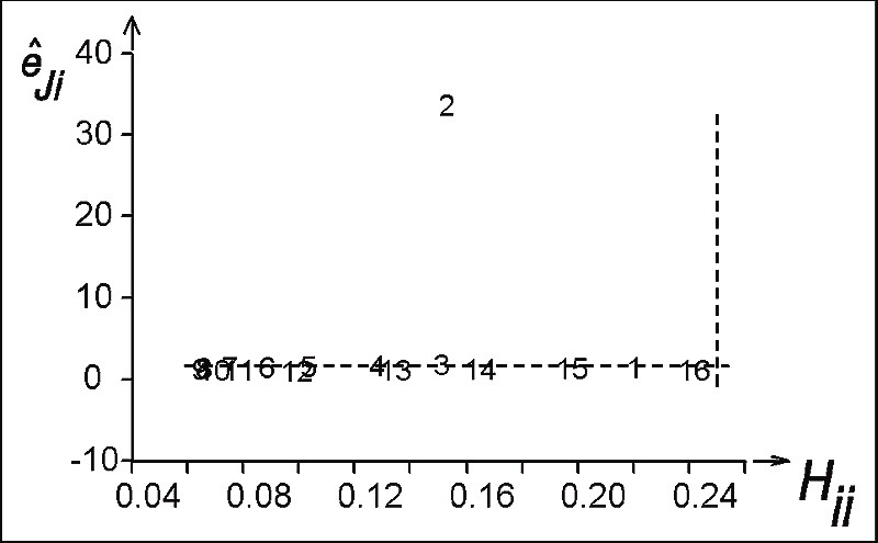
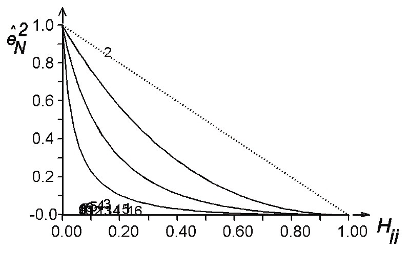
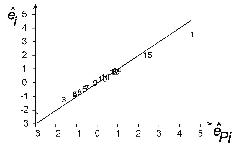
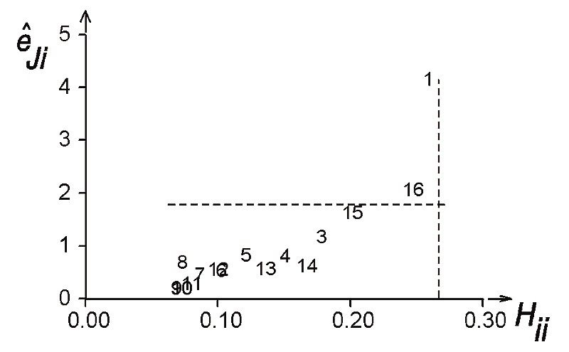
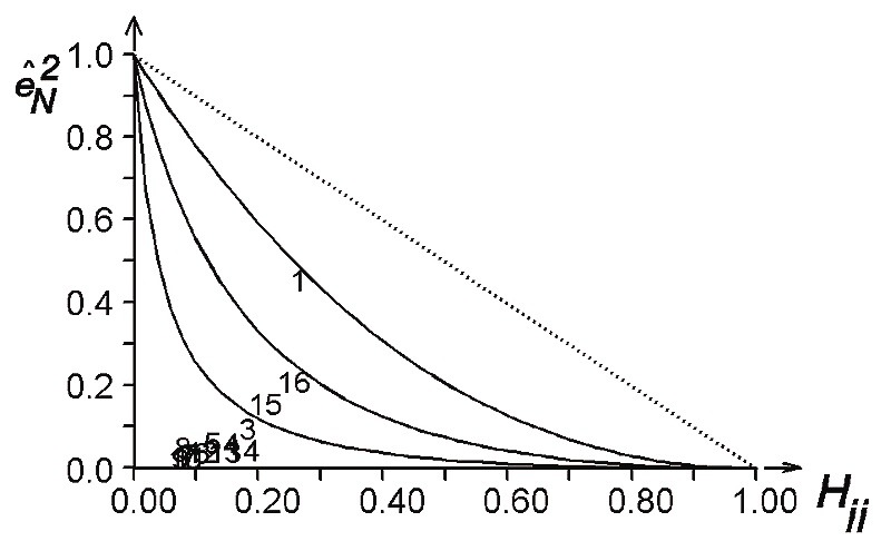
Fig. 5 Diagnostic plots indicating influential points based on residual and hat matrix elements for the original data set of Example 1: (5a) Graph of predicted residuals, (5b) Williams graph, (5c) Gray s L-R graph, and these plots after excluding point no. 2 from data: (5d) Graph of predicted residuals, (5e) Williams graph, (5f) Gray s L-R graph.

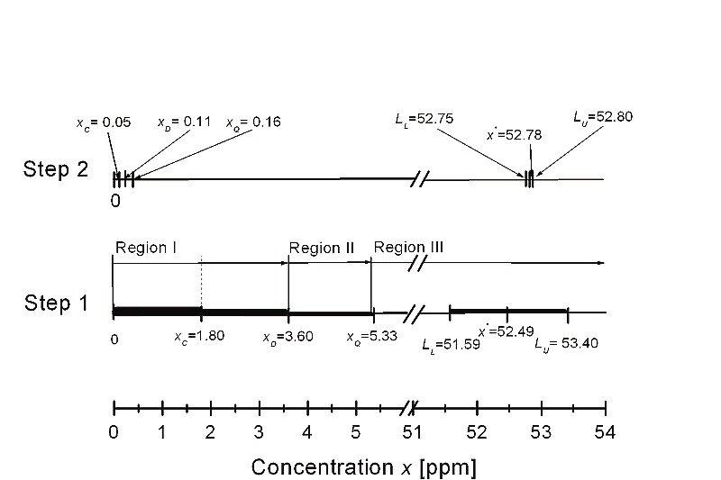
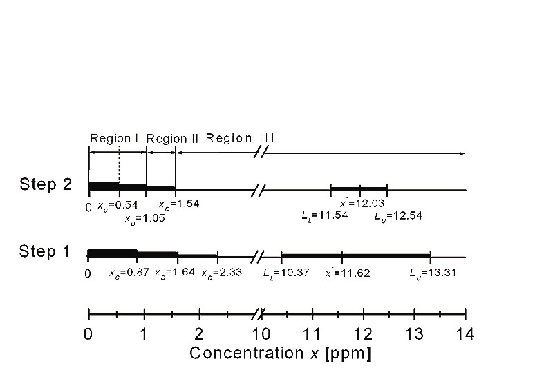
Fig. 6 The three principal analytical regions of calibration precision limits and the point x* and interval estimates [LL, LU] of the unknown concentration in dependence on regression triplet analysis for Example 1 and Table 1 where Region I means “the region of unreliable detection”, Region II means “the region of qualitative estimation”, and Region III means “the region of quantitative estimation of unknown concentration”. Calibration precision limits xC, xD and xQ, and x* with [LL, LU] are calculated. In Step 1 the original data with all outliers are fitted with the straight line using OLS while in Step 2 the data without the three outliers nos. 1, 2, and 16 and using OLS.

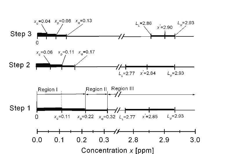
Fig. 7 The three principal analytical regions of calibration precision limits and the point x* and interval estimates [LL, LU] estimates of the unknown concentration in dependence on regression triplet analysis for Example 2 and Table 2. Description of regions is the same as in Fig. 6: in Step 1 the original data with all outliers are fitted with the straight line using OLS, in Step 2 the same as in Step 1 but using the IRWLS method, and in Step 3 the original data without 8 outliers and using the IRWLS method were fitted with the straight line.

Fig. 8 The three principal analytical regions of calibration precision limits and the point x* and interval estimates [LL, LU] of the unknown concentration in dependence on regression triplet analysis for Example 3 and Table 3. Description of regions is the same as in Fig. 6: in Step 1 the original data with all outliers are fitted with the straight line using IRWLS, and in Step 2 the original data are fitted with the quadratic spline and using IRWLS.