")
")
Published in:
M. Meloun, J. Militký, M. Hill, R. G. Brereton, Crucial Problems in Regression Modelling and Their Solutions, The Analyst, 127, 433 - 450 (2002).
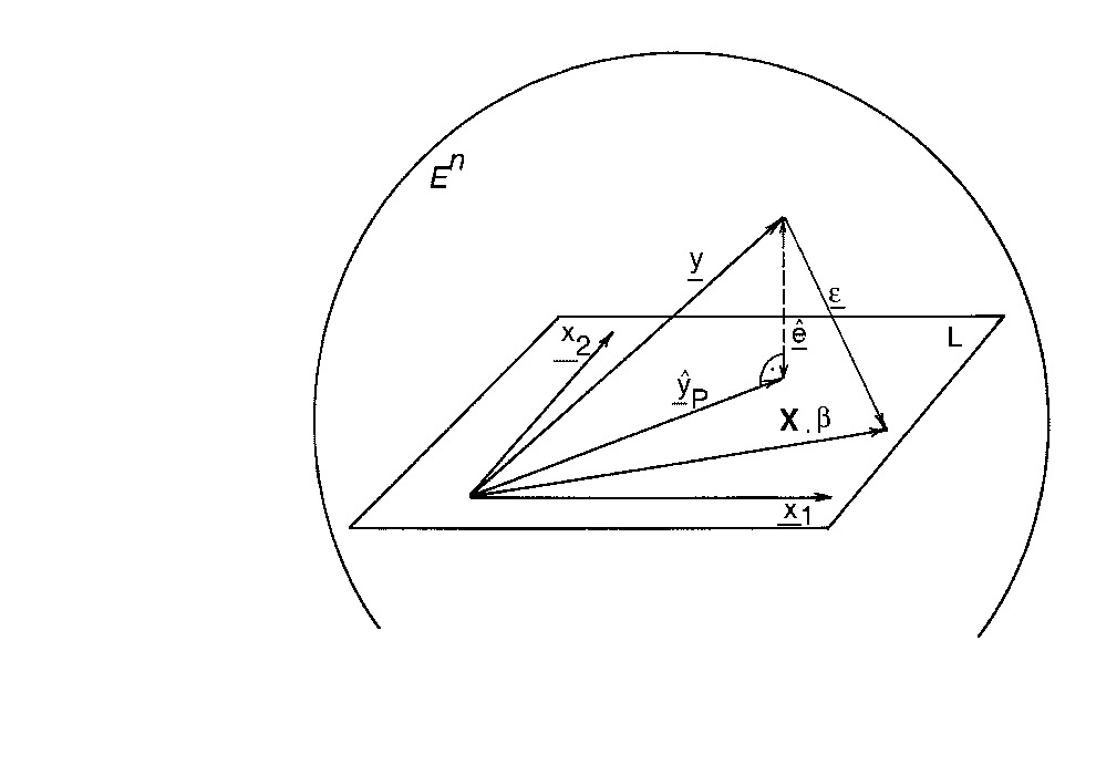
| Data131.xls | Fig. 1.1 Geometric illustration of a linear regression model for two independent variables. |
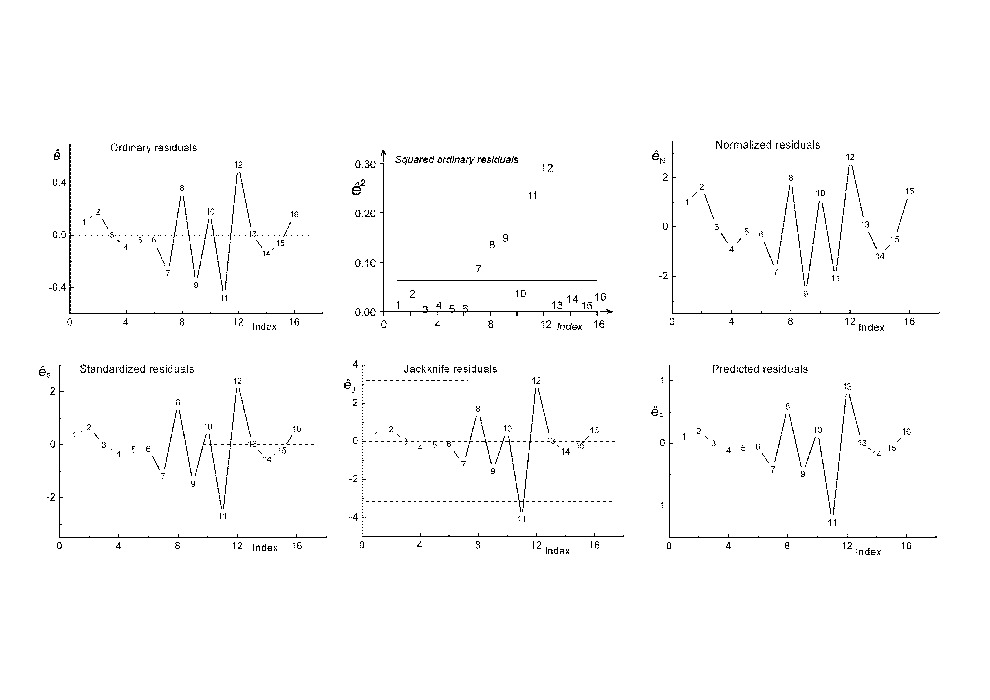
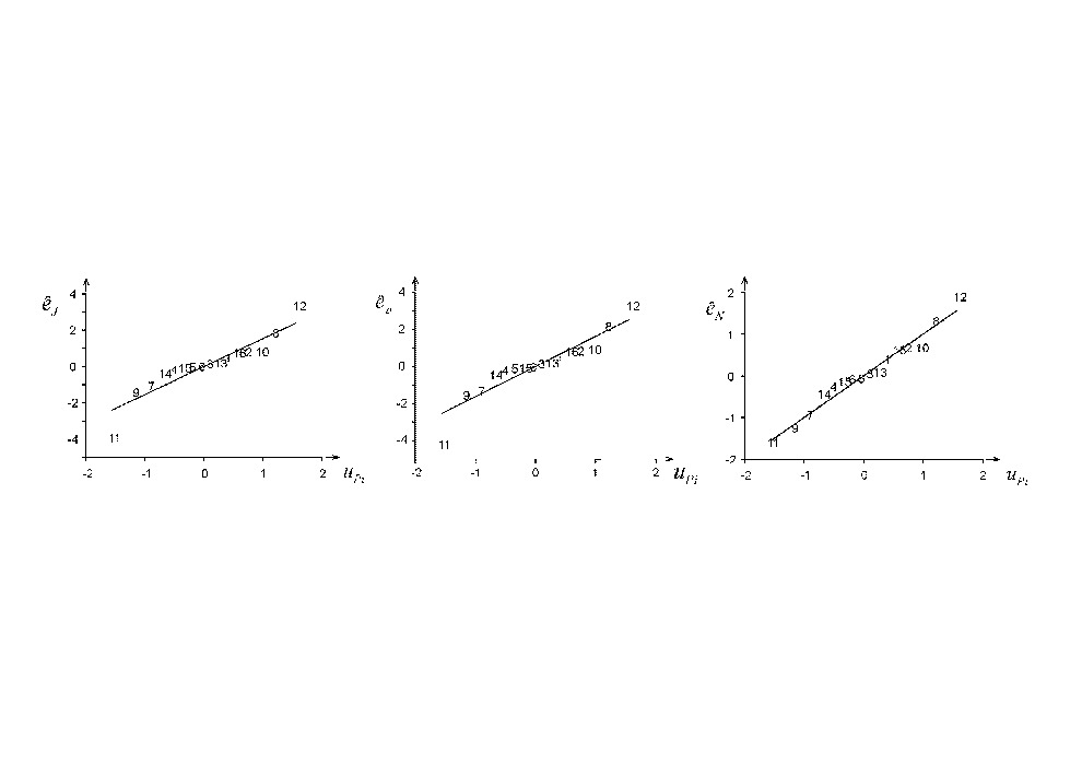
| Fig. 1.2 Index graphs of various residuals for the data set of Example 1: (a) Ordinary residuals; (b) Square of ordinary residuals; (c) Normalized residuals; (d) Standardized residuals; (e) Jackknife residuals; (f) Predicted residuals | |
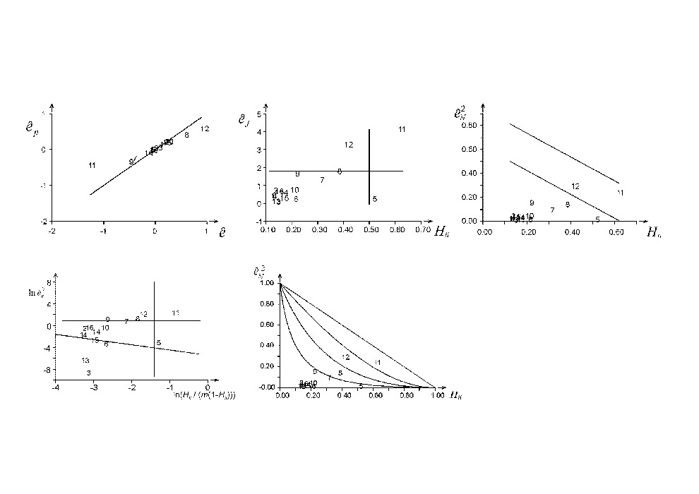
| Fig. 1.3 Diagnostics based on residual plots and hat matrix elements for the data set of Illustrative example 1.1: (a) Graph of predicted residuals, (b) Williams graph, (c) Pregibon graph, (d) McCulloh and Meeter graph, (e) Gray’s L-R graph | |
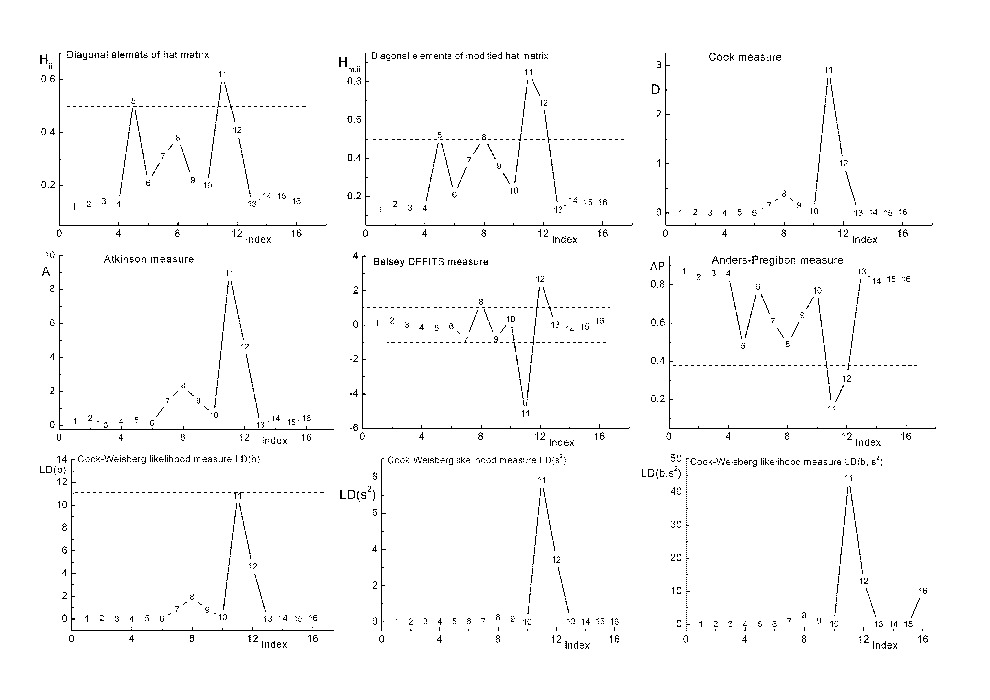
| Fig. 1.4 Index graphs of vector and scalar influence measures: (a) Diagonal elements of the hat matrix; (b) Diagonal elements of the modified hat matrix; (c) Cook measure; (d) Atkinson measure; (e) Belsey’s DFFITS measure; (f) Anders-Pregibon measure; (g) Cook-Weisberg likelihood measure LD(b); (h) Cook-Weisberg likelihood measure LD(s2); (i) Cook-Weisberg likelihood measure LD(b, s2) | |
| Fig. 1.5 Rankit Q-Q graph of (a) jackknife residuals., (b) predicted residuals, (c) normalized residuals | |
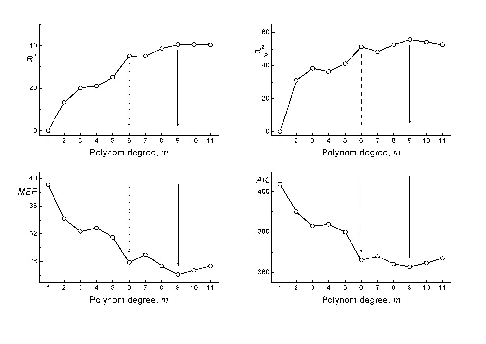
| Fig. 2.1 The search for an optimal polynomial degree m leads to one local (dashed line) and one global extreme (full line) when the following dependences and the ordinary least squares OLS were used: (a) the determination coefficient R2 on m, (b) the predicted coefficient of determination R2P on m, (c) the mean error of prediction MEP on m, (d) the Akaike information criterion AIC on m | |
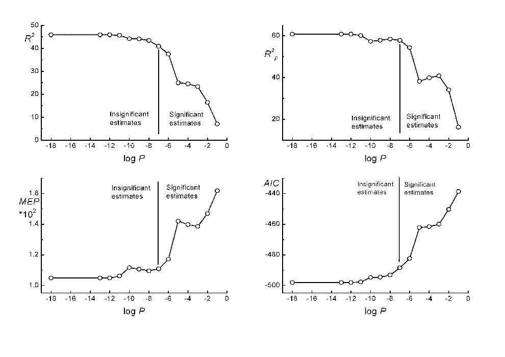
| Fig. 2.2 The search for the GPCR optimal criterion value P separates statistically significant and insignificant parameter estimates when the method of generalized principal component was used: (a) the determination coefficient R2 on P, (b) the predicted coefficient of determination R2P on P, (c) the mean error of prediction MEP on P, (d) the Akaike information criterion AIC on P | |
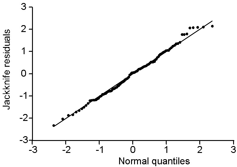
| Fig. 2.3 The rankit Q-Q graph of jackknife residuals proves the normality of the random errors in the transformed dependent variable y0.13 | |
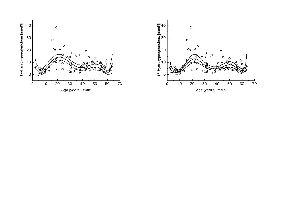
| Fig. 2.4 Nonlinear regression of the 8th degree polynomial of the age-dependence of 17-hydroxypregnenolone when (a) the original variable y was used, (b) the transformed variable y0.13 was used | |
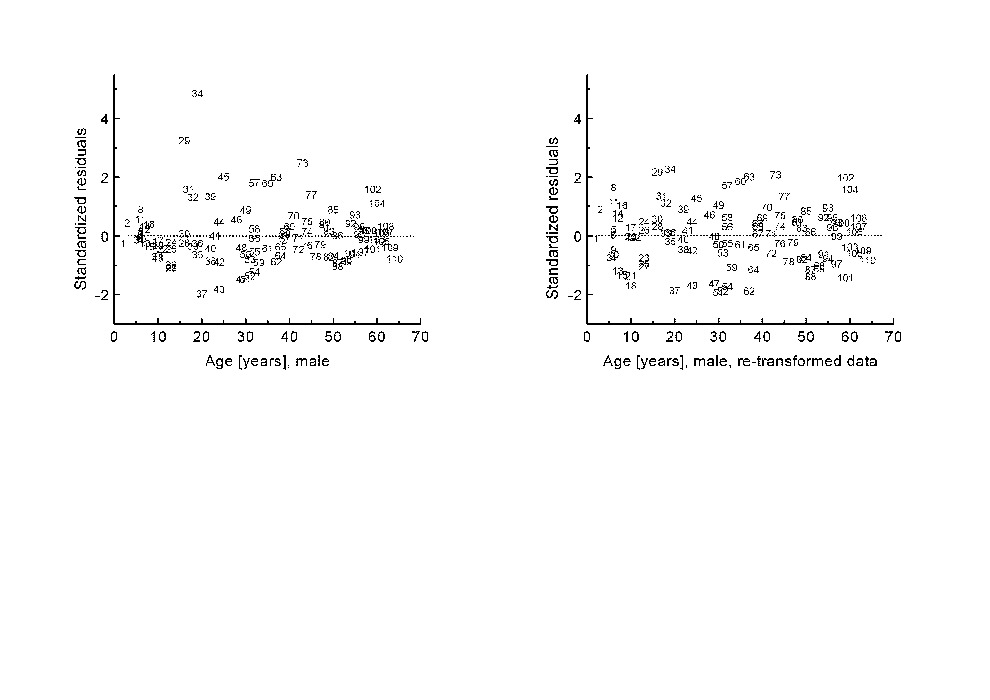
| Fig. 2.5 The scatter plot of standardized residuals on age x when (a) the original variable y was used, (b) the transformed variable y0.13 used | |
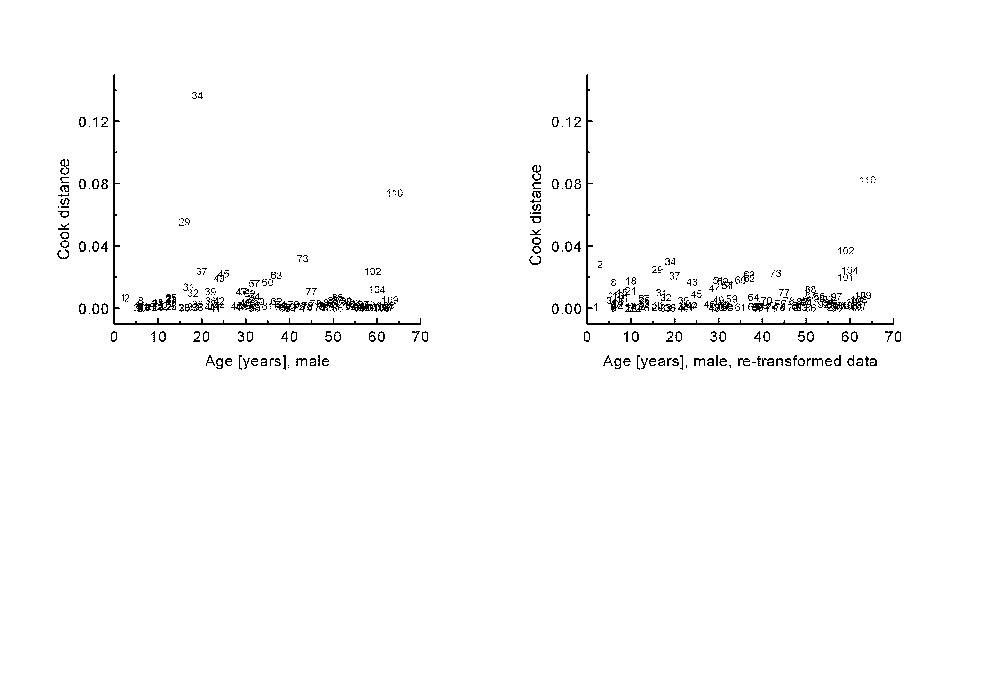
| Fig. 2.6 The scatter plot of Cook distance D on age x when (a) the original variable y was used, (b) the transformed variable y0.13 was used |