")
")
Published in:
M. Meloun, J. Militký: Detection of Single Influential Points in OLS Regression Model Building, Anal. Chim. Acta, 439, 169 - 191 (2001).
|
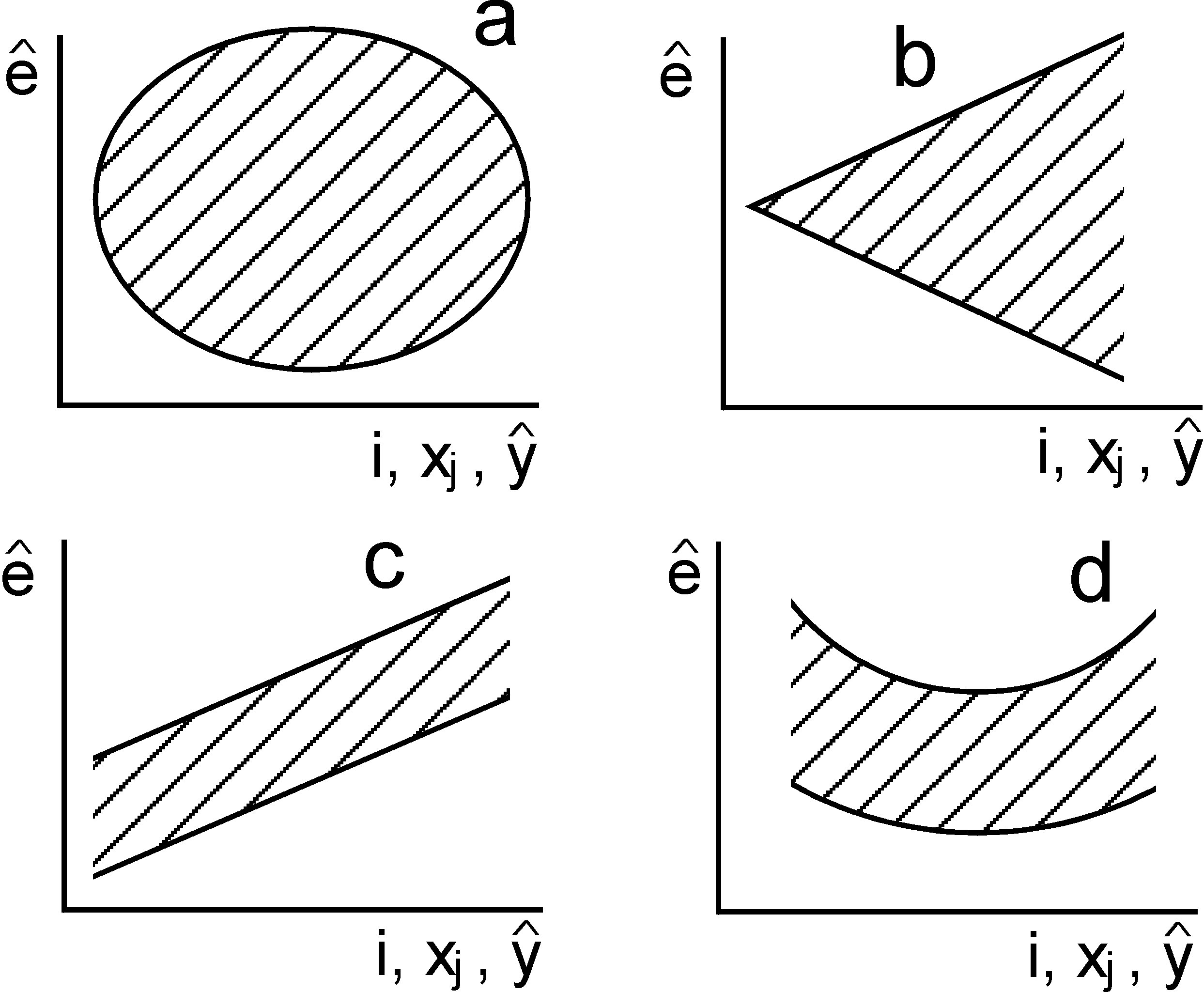
Fig. 1 Possible shapes of residual plots: (a) random pattern shape, (b) sector pattern shape, (c) band shape, (d) nonlinear curved band shape. |
|
|
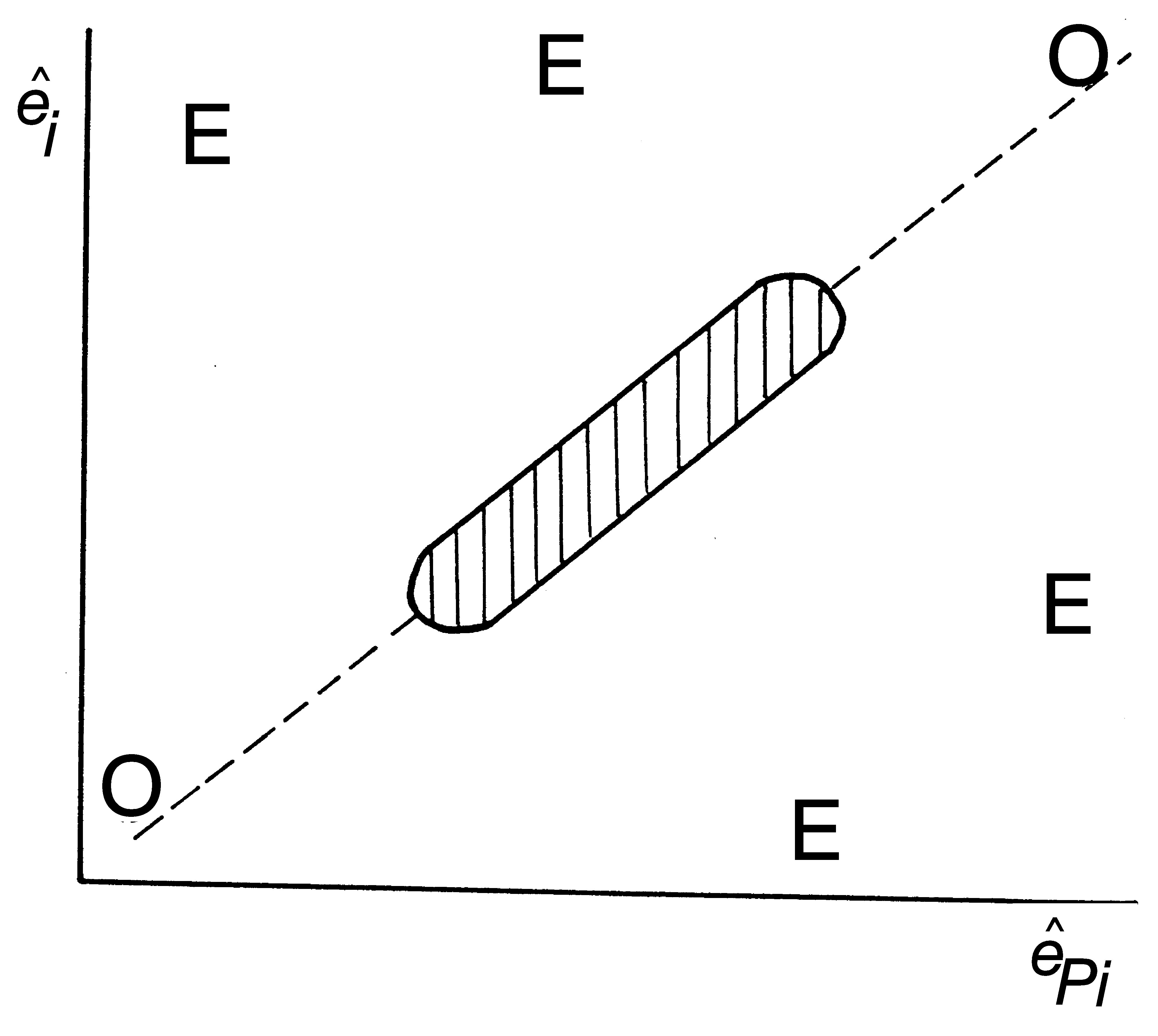
Fig. 2 Graph of predicted residuals: E means a high-leverage point and O an outlier; outliers are far from the central pattern on the line y = x. |
|
|
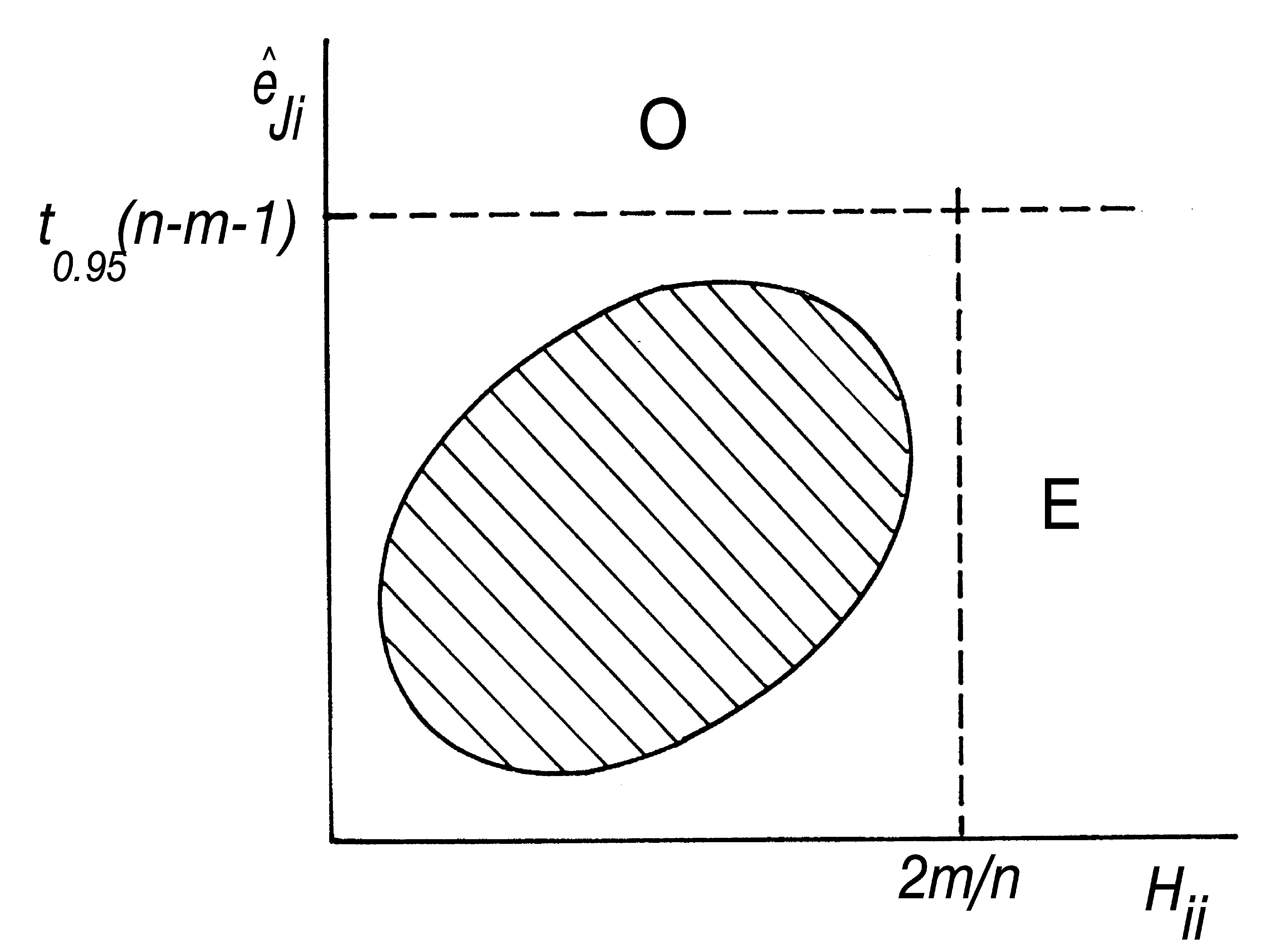
Fig. 3 Williams graph: E means the leverage point and O the outlier; the first line is for outliers, y = t0.95 (n - m - 1), the second line is for high-leverages, x = 2m/n. |
|
|
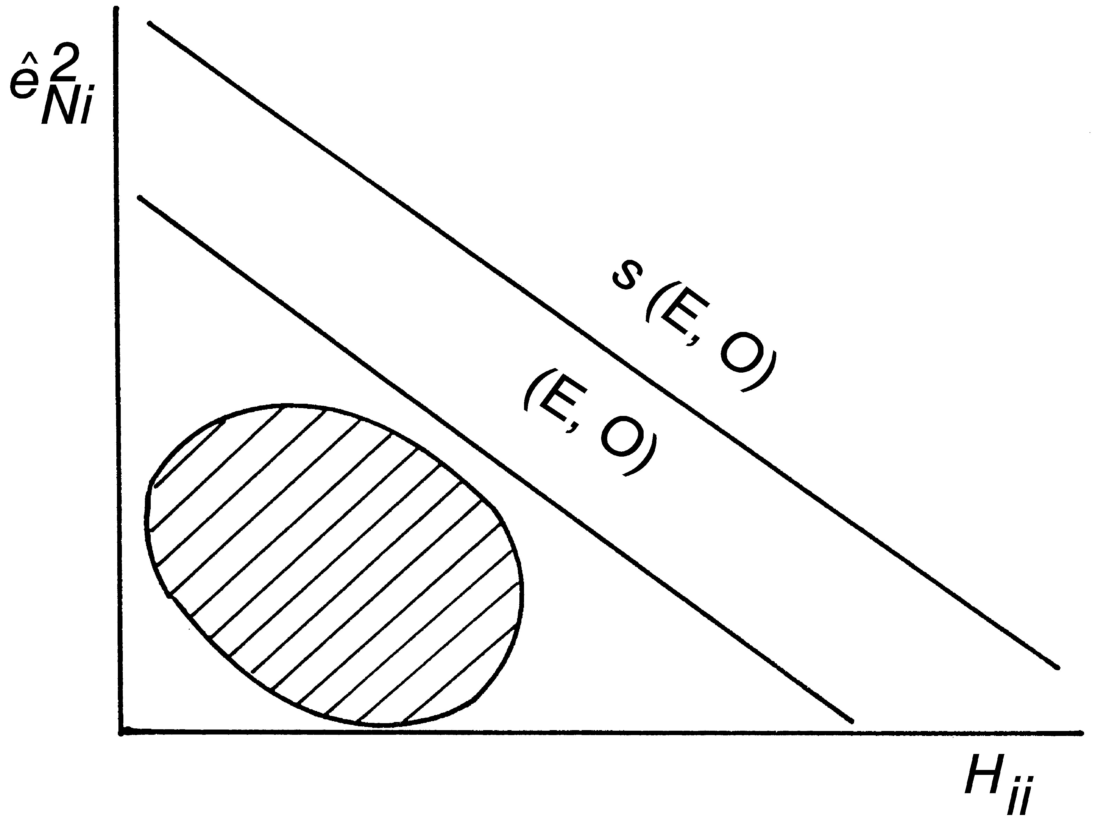
Fig. 4 Pregibon graph:(E, O) are influential points, and s(E, O) are strongly influential points; two constraining lines are drawn, y = -x + 2(m + 1)/n, and y = -x + 3(m + 1)/n, the strongly influential point is above the upper line; the influential point is between the two lines; |
|
|
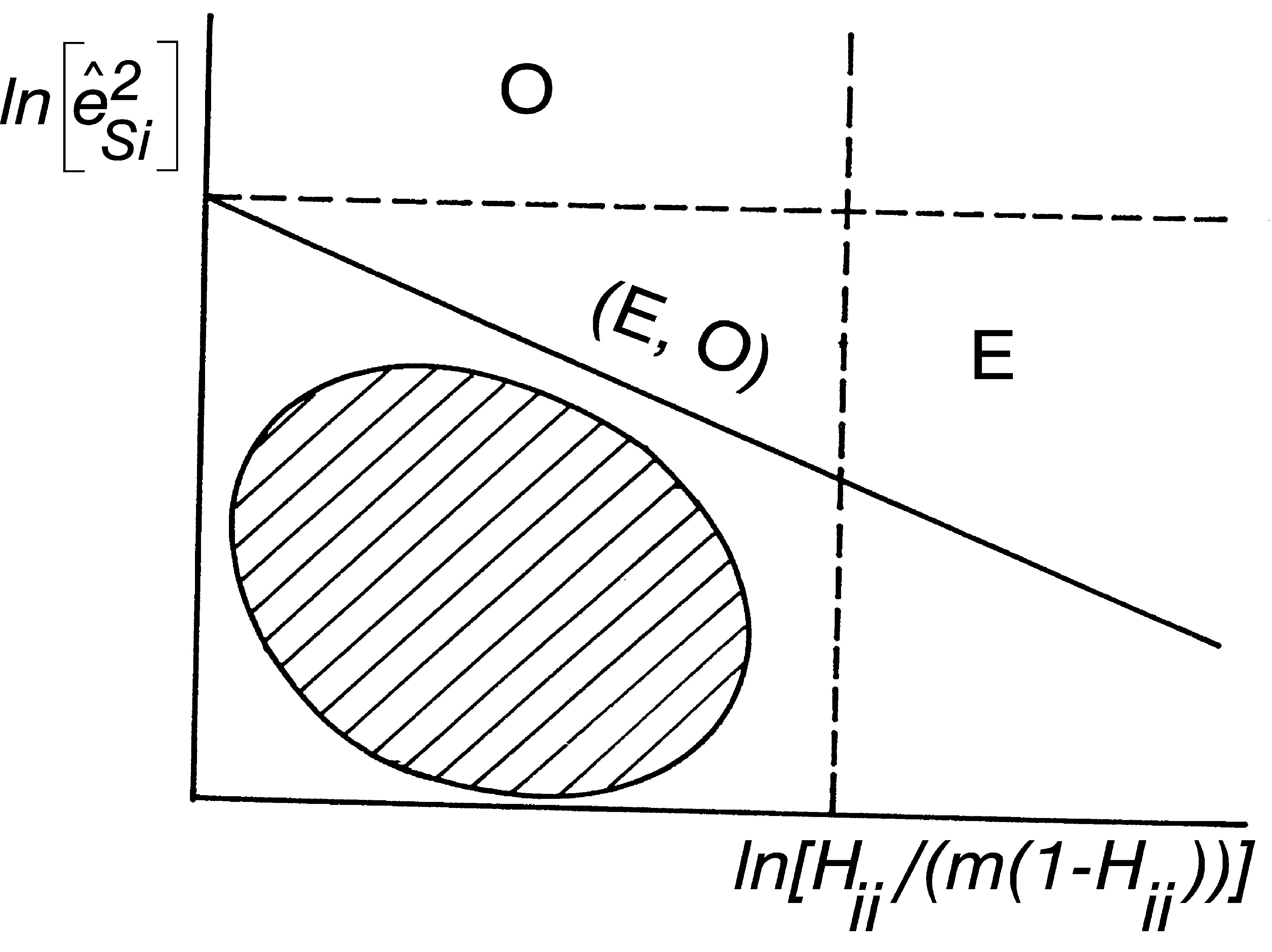
Fig. 5 McCulloh and Meeter graph: E means a high-leverage point and O an outlier, (E, O) an influential point; the 90% confidence line is for outliers, y = -x - ln F0.95(n - m, m) while the boundary for high-leverages is x = ln[2/(n - m) × (t20.95(n - m)]. |
|
|
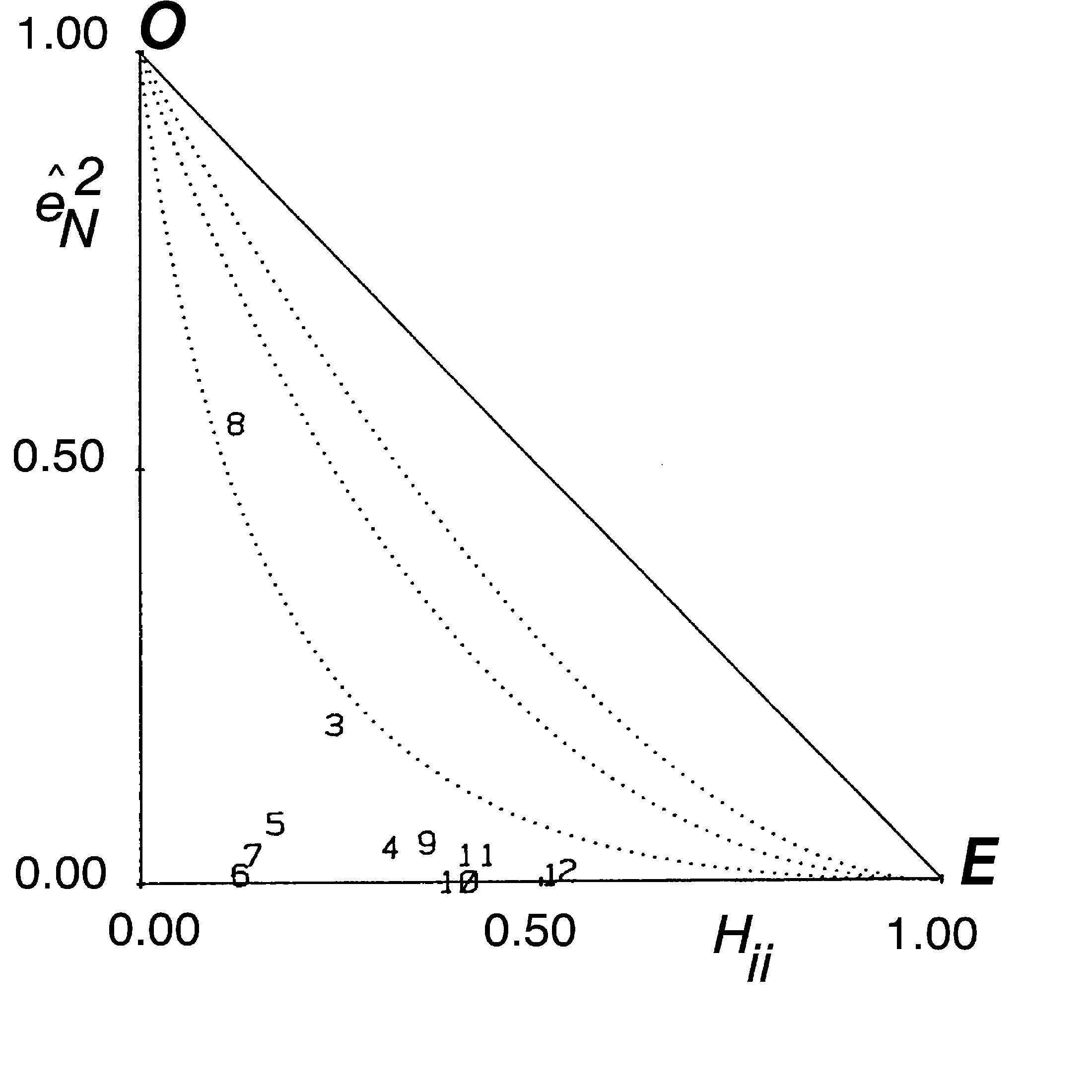
Fig. 6 L-R graph: E means a high-leverage point and O an outlier, and digits in the triangle stand for the order index i of the response (dependent) variable yi; points towards to the part are outliers while towards the right angle of triangle are high-leverages. |
|
|
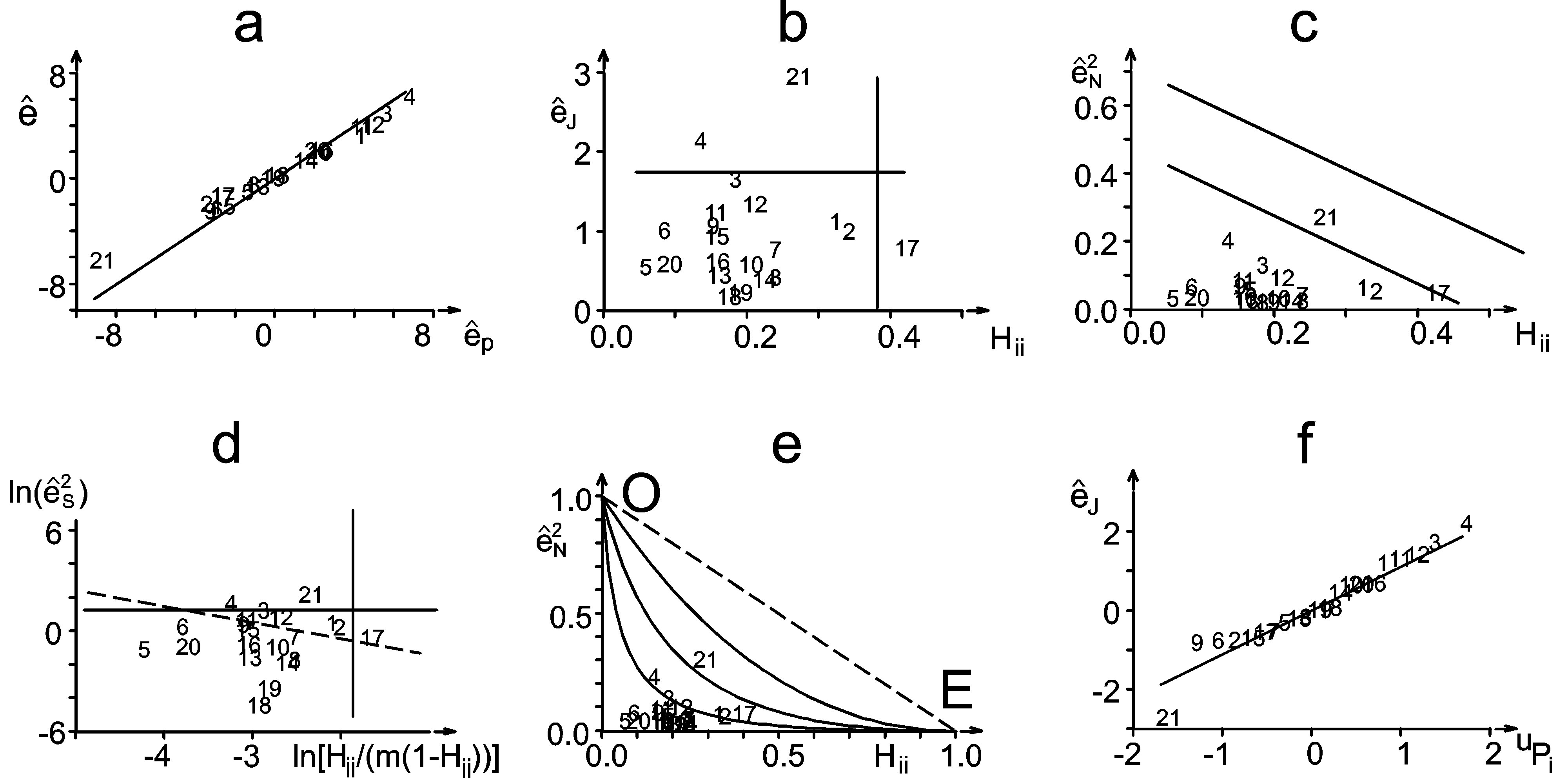
Fig. 7 Diagnostics based on residual plots and hat matrix elements for stackloss data: (a) graph of predicted residuals, (b) Williams graph, (c) Pregibon graph, (d) McCulloh and Meeter graph, (e) Gray L-R graph, (f) rankit Q-Q graph of jackknife residuals. |
|
|
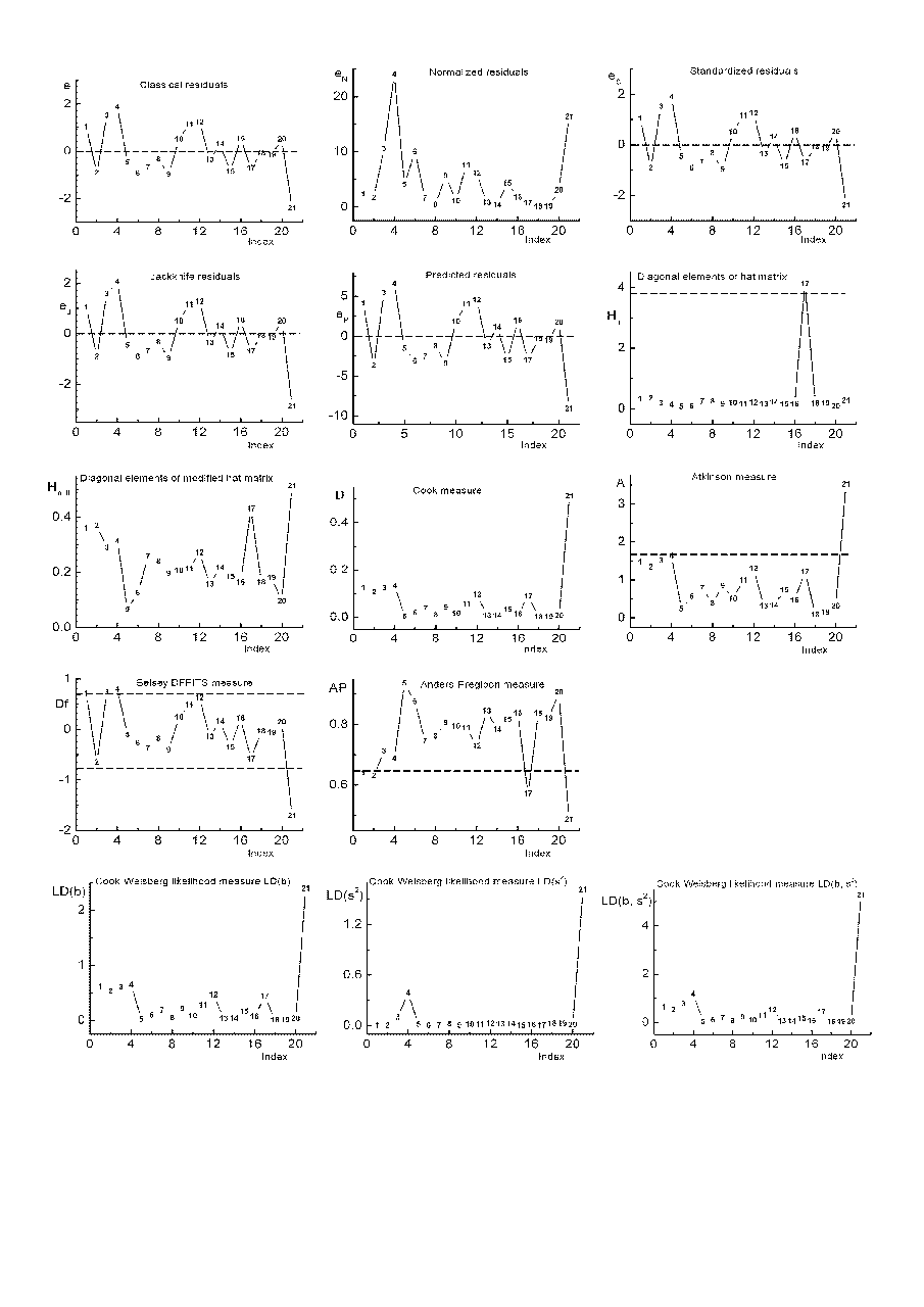
Fig. 8 Index graphs of various residuals and vector and scalar influence measures for stackloss data: suspicious points (SP) are points which obviously differ from the others; influential points (IP) are points which are detected and are separated into outliers and high-leverages |
|
|
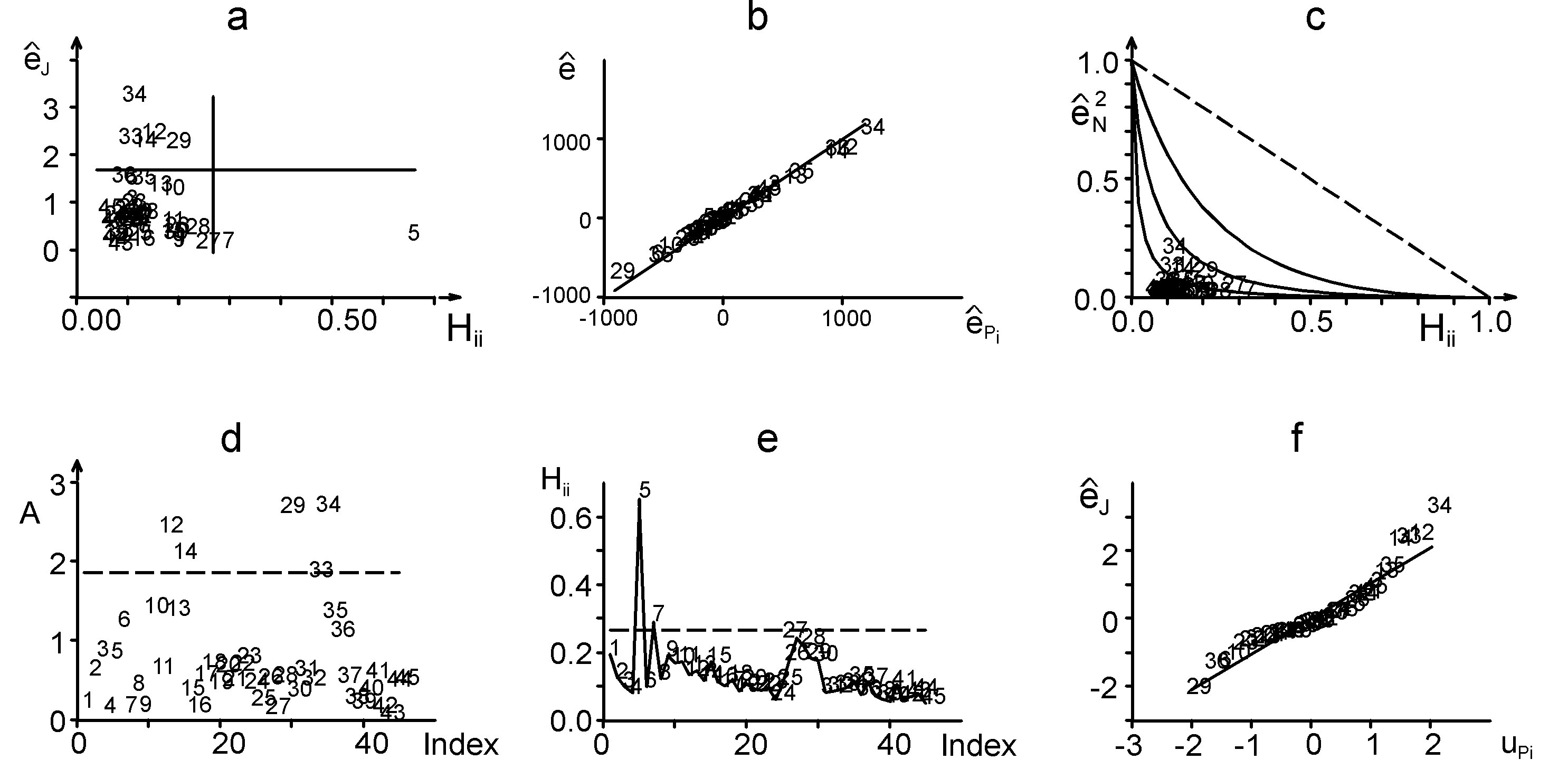
Fig. 9 Selected IP-diagnostics plots for the detection of influential points in aerial biomass data: (a) Williams graph, (b) graph of predicted residuals, (c) Gray L-R graph, (d) index graph of Atkinson measure, (e) index graph of diagonal elements of the hat matrix, (f) rankit Q-Q graph of jackknife residuals. |
|
|
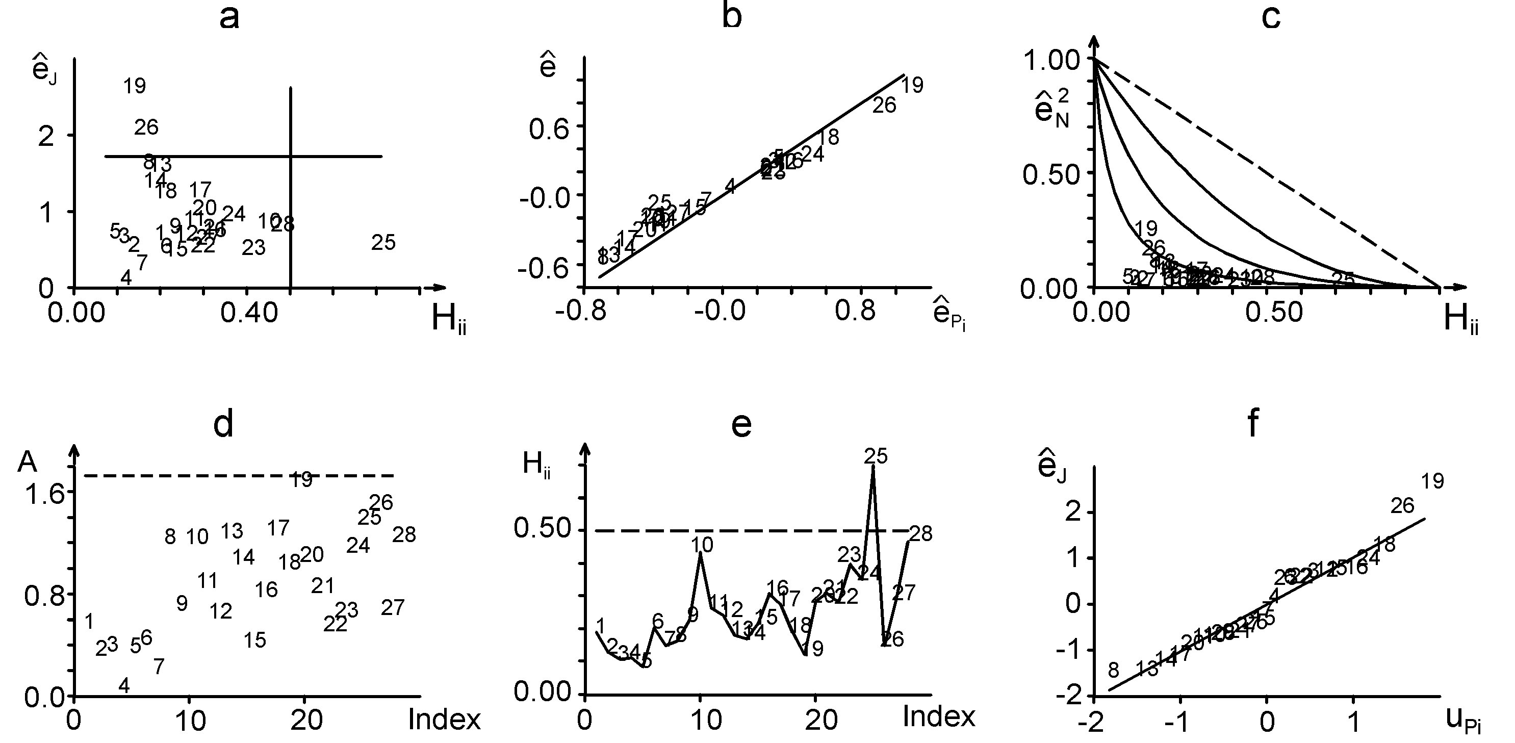
Fig. 10 Selected IP-diagnostics plots for the detection of influential points in structure-activity data: (a) Williams graph, (b) graph of predicted residuals, (c) Gray L-R graph, (d) index graph of Atkinson measure, (e) index graph of diagonal elements of the hat matrix, (f) rankit Q-Q graph of jackknife residuals. |